Wednesday, June 30, 2021

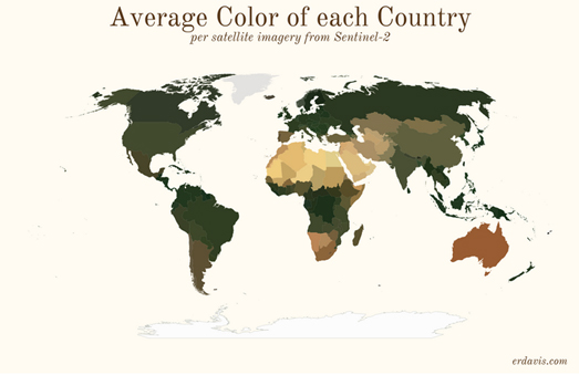
The Average Color of the Earth

Last week Erin Davis published a series of interesting maps showing the average colors of countries around the world based on Sentinel satellite imagery. The Average Colors of the World includes maps of each continent and a map of the world on which each country is colored based on its average satellite color.

The results are very interesting and clearly reveal the Sahara desert in Africa and the Australian outback. Erin's map showing the average color of each county in America also clearly visualizes the deserts of the Southwest and the greenery of the Midwest breadbasket.  

Erin doesn't provide much information about the satellite imagery used to determine the average colors for each country, beyond that they were sourced from Sentinel-2.I can't help thinking if you sourced a different set of satellite imagery you would probably arrive at different average colors for each country. You would probably also achieve different average colors for each country of the world if you used satellite imagery taken in the different seasons of the year or taken at different times of the day. It seems obvious that the average color of a country will be very different in the summer than it is in the winter.


Mindhue Studio has also determined the average color of each continent based on satellite imagery. In Average Continent Colors each continent is given an average color as derived from "a NASA true-color cloudless satellite montage of the world". 

Comparing Mindhue Studio's average color of Australia with Erin Davis's average color for the country we can see that there is a quite a difference between the two average colors. This may have something to do with the different methodologies used to determine the average color. However it is also likely to be influenced by differences in the sourced satellite imagery. Arriving at a definitive average color for a country is likely to be impossible as the 'color' of a country is dynamic and changes with the seasons (and probably with global heating). However to get a more accurate average color we could sample satellite imagery taken throughout the course of a year ...

The Average Earth Map 2020 is an interactive satellite map which is constructed from imagery captured by NASA satellites over the course of last year. The reason why it is called the 'average' Earth map is because each pixel on the map shows the average color of that location over the whole of 2020.

In order to create the map cartocalypse used 365 daily satellite composite images of the Earth. All 365 satellite images (one for every day) were then merged together and the average color of each pixel was determined. The result is a satellite view of the Earth which shows cloud patterns, permafrost and prevailing wind patterns. Although, as cartocalypse warns, the map isn't "a true representation of the typical weather or cloud cover throughout the year". The daily satellite images were captured at the same time every day by NASA - so the rest of the day isn't a part of this 'average' Earth image. 

You can read more about how the Average Earth Map was created, including how the satellite images were downloaded, processed and analyzed on this Satellite Composite of Earth 2020 blog post. This isn't the first time that cartocalypse has created an average Earth map. You might also enjoy his interactive Average Earth from Space 2018 map.

The 3D Map of Bonn

The city council of Bonn has released an impressive 3D map of the German city. Bonn in 3D was created from around 10,000 aerial photos, resulting in a beautiful photo-realistic virtual model of the former capital of West Germany.

The map menu allows you to access a number of map features. The 'Sehenswürdigkeiten' option provides links to tourist attractions in Bonn, which is particularly useful if you want to view some of the city's most impressive landmarks on the 3D map. The 'Überblicke' option is also an impressive feature of the 3D map, allowing you to virtually experience the views from some of the city's hills and tallest buildings on the 3D map. The 'Natur und Landschaft' option allows you to view the locations of the city's nature reserves and parks.

The 'Kartenauswahl' link in the map menu allows you to explore the aerial photos of the city which were used to create the 3D map. To create the 3D map oblique aerial photographs of the city were taken from four different directions. If you select the Kartneauswahl link you can explore any location in the city as seen from four different oblique aerial views.

Tuesday, June 29, 2021

Canada's Residential School Map

From the 19th Century until the end of the 20th Century Canada's Indian residential school system existed to separate Indigenous children from their families in order to remove them from the influence of their own culture and to 'assimilate' them into Canadian culture. The system existed for more than a century, during which time around 150,000 children were placed in residential schools nationally. The children were forced to convert to Christianity and were not allowed to speak or learn their own native languages.

CBC's Residential Schools map allows you to search for the residential school nearest to you. Enter a Canadian address into the map and it will show you the nearest residential school to that address and when the school was operational.

The last residential school was closed in 1996. However that doesn't mean things are now perfect for Indigenous people in Canada. From 2001 to 2015 the homicide rate for Indigenous women in Canada was nearly six times as high as the homicide rate for other women.

The Native Women's Association of Canada (NWAC) has published an interactive map of cases of missing and murdered Indigenous women and girls. The Safe Passage map includes over 300 locations where a missing Indigenous woman or girl was last seen or where remains have been found. The map is being used to collect data and help identify patterns of violence in geographic areas.

Individual cases are shown on the map using colored markers showing whether the case relates to a homicide, a missing person or a suspicious death. The map also includes a heat-map view showing where the number of cases of missing and murdered Indigenous women and girls are most dense.

London's New Constituencies

The Boundary Commission for England recently released its 2023 Review of Parliamentary Constituencies. This review includes its proposals for changing the parliamentary constituencies in England. Under these proposals the number of constituencies in London will increase from 73 to 75. 

My Gerrymander London map shows the boundaries of the recommended 75 London constituencies. Some of the boundaries for these new recommended electoral areas are significantly changed from the existing constituency boundaries. You can respond to these new recommendations from the Boundary Commission during the consultation period, which lasts until 2nd August 2021. 

On the map each of the recommended constituencies is colored by its Polsby-Popper score. The Polsby-Popper test is a mathematical formula for calculating how compact an electoral district is in order to detect for possible gerrymandering. The general assumption is that the more compact a constituency is the less likely it has been gerrymandered.

Based on my analysis Bethnal Green and Stepney has the highest Polsby-Popper score, so is therefore the constituency which is least likely to have been gerrymandered. Brent Central has the lowest Polsby-Popper score, so it is the constituency in London which is most likely to have been gerrymandered.

On my map I have also tried to calculate which party would be elected in each of the 75 proposed new constituencies. There is very little difference in the average Polsby-Popper scores for each of the three main political parties in London. So although some constituencies, such as Brent Central, are not very compact there is little evidence that the Boundary Commission has attempted to gerrymander London's proposed new constituencies in favor of any of the political parties.

Monday, June 28, 2021

Massacres of the United States

Massacres in the United States is a fascinating but gruesome map showing the locations of the worst massacres in the history of the United States. The history of the United States is of course littered with many acts of extreme violence, from the slaughter of Native Americans by settlers to the massacre of African Americans throughout its short history.

According to the map the largest massacre in U.S. history occurred in the 1850's in California. Soon after California became the 31st state (in 1850) legislation was introduced giving settlers the right to organize lynch mobs and kill Native Americans. It is estimated that between 1856-1859 over 1,000 Yuki people were killed by white settlers. 

On the Massacres in the United States interactive map the colored markers are sized to show the number of people killed in each massacre. The colors of the markers indicate the massacre 'category' (Native American, African-American, Labor Unions etc). If you click on a category in the map sidebar you can filter the map to show only massacres from that category. For example if you select 'Native Americans' you can see that 19th Century California witnessed a succession of massacres carried out against the indigenous people.

Only massacres with 5 or more victims are shown on the map. The data for the map comes from Wikipedia, so only massacres with a Wikipedia entry are shown on the map.

The Tour de France Live Tracking Map

The Tour de France Live Tracking is the official Tour de France live tracking map which allows you to follow the world's premier cycle race in real-time on an interactive map. The map shows the live position of the front of the race the peloton and the back of the race. 

A yellow line shows the stage route of the race on the map. If you zoom in on the markers on the map you can view them moving in real-time. These numbered markers are colored to show you where the yellow, red polka dot and green jerseys are currently located.You can also click on these markers to view the individual riders in each group. 

If you click on the small inset altitude map you can view live data from the race. This data includes the current time difference between the front of the race and the peloton, the distance left in the race, the average speed and the current weather conditions. This live data view includes a real-time commentary stream, which provides real-time overview highlights from the race.

Le Monde has created a fascinating map showing how often the Tour de France has visited each département in France. How Many Times has the Tour de France Visited Your Département? provides a choropleth view of the départements most used in the world's greatest bike race.

This map includes a timeline tool which allows you to view the tour's favorite locations for any period in the race's history. As you can see in the screenshot above (showing every year of the Tour de France) the départements around the edge of France tend to see the Tour de France more than the départements in the country's interior.

This pattern was even more pronounced in the earliest years of the Tour de France. Adjust the timeline on the map to view the first ten years of the race (1903-1913) and that ring around the external border of France is even more pronounced.

The two départements which have been most ignored by the Tour de France don't actually feature on this map. The two départements on the island of Corsica have only seen the race once, when it visited in 2013. The least visited département on the mainland of France is Indre, which has only featured in 8 of the 104 Tour de France races.

The Haarlem Road Plotters

Over the last few years I've spent a lot of time curating building age maps from around the world. These are interactive maps which color individual buildings in a town or city by year of construction. A building age map can be a very effective way to visualize how a city has developed over time.

Another way to visualize the development of a city is to create a street age map.Streets in Haarlem is an interesting map which shows the age of construction of all the streets in the Dutch city of Haarlem. On this map colored circles are used to indicate the year of each road's inception.As you might guess the map seems to show that the city's oldest streets are in the center and that the streets tend to become more recently constructed as you move from the center to the outer suburbs.

You can also click on individual streets on the map to learn about the meaning behind the street's name (for example, who it was named for). The map uses information about street names and construction dates from Wikidata. 

An example of a Wikidata entry for a street in Haarlem is Mollerusweg (Mollerus Road), a road named after Johan Cornelis Mollerus and constructed in 1978. The Streets in Haarlem map includes a drop-down menu which allows you to view maps for many other Dutch towns. Unfortunately Wikidata doesn't have data on the construction dates of streets in many Dutch towns so most of these maps don't visualize the construction dates of the city's streets.However these maps do include the 'named after' data. So these maps can still be used to discover who individual streets were named for. 

If you have an interest in who streets are named after - particularly in the disparity in the number streets named for men and women in cities around the world - then you should browse through the toponym tagged posts on Maps Mania. 

Saturday, June 26, 2021

How Slow Will Your Post Be?

In March the Postmaster General Louis DeJoy proposed that the US Postal Service change the delivery times of first class mail from one-to-three days to one-to-five days. He says the proposals would save the USPS $160 billion over the next decade.

The Washington Post has mapped out how the Postmaster General's plans will effect your post. In DeJoy’s USPS slowdown planwill delay the mail. What’s it mean for your Zip code? the Post has created before and after maps showing the percentage of mail delivered in 2, 3, 4 or 5 days. It also has an interactive map which allows you to enter your zip-code to see how long your mail will take to get delivered to different areas of the country.

Under the new delivery proposals states west of the Rocky Mountains and areas such as southern Texas and Florida will be effected the most. For example 60% of first-class deliveries to Florida will take longer to arrive.

In 1899 there were five times as many post offices in the United States as there are McDonald's restaurants today. The Gossamer Network is an interactive map which visualizes the extraordinary expansion of the U.S. Post during the 19th Century. The map also provides a detailed overview of how the Post Office network was able to conquer the west over the course of the second half of the 19th Century.

The 3D Glastonbury Festival Map

This weekend thousands of people should be enjoying five days of music and contemporary performing arts at the Glastonbury Festival. Unfortunately for the second year running the festival has had to be cancelled. If you are missing the festival experience this weekend then you can console yourself by visiting the V&A museum's 3D Glastonbury map.

Mapping Glastonbury is an interactive 3D map made by the Victoria and Albert Museum for its Glastonbury Weekender exhibition. The map uses the real topography of Worthy Farm to create an immersive 3D experience, which allows you to explore how the festival has grown over the decades and get a small taste of the Glastonbury experience. 

Mapping Glastonbury includes a timeline which allows you to view 3D maps of the festival site for each decade from the 1970s to the 2010s. This allows you to visualize how the festival has grown from a relatively small event attended by 1,500 people to the huge festival site of the present, which is normally attended by around 175,000 people.

If you double-click on the 3D map you can zoom in and explore the different areas of the festival site, including the Pyramid Stage, the Green fields and the Unfairground. You can also click on the floating nodes on the map to access photographs, soundscapes and videos of the festival from the V&A's own Glastonbury Festival Archive.

Friday, June 25, 2021

230 Years of Mapping

230 years ago, on the 21 June 1791, the Board of Ordnance was founded in order to survey the southern coast of England to help protect Britain from possible French invasion. 230 years later the Board of Ordnance is still going strong, although these days it goes by the name Ordnance Survey.

To celebrate its 230th birthday the Ordnance Survey has released Ordnance Survey Mapping Through the Centuries, an Esri story map which both recounts the history of Britain's national mapping agency and also allows you to explore some of its celebrated maps. These maps include the Board of Ordnance's very first map of Kent and the southern coast of England closest to France.

The Ordnance Survey Mapping Through the Centuries story map also explores the history of mapping over the last two hundred years and the technological changes in cartography during that time (from trig pillars to orbiting satellites)

During lockdown I have had a lot of fun exploring historical Ordnance Survey maps. In particular I have used old Ordnance Survey maps to explore how my neighborhood has developed and changed over the last 150 years.Using vintage Ordnance Survey maps has given me a far greater understanding of how my neighborhood has changed over the last two hundred years and also helped make my local walks far more interesting.

The National Library of Scotland's Ordnance Survey Map Finder is a great way to find and view vintage Ordnance Survey map of British towns and cities. Using the library's online map you can find old Ordnance Survey maps dating back as far as the 1860s. By exploring your neighborhood on these historical maps you can learn a lot about how an area has developed over time and about some of the local historical landmarks and buildings which have been replaced by more modern developments.

Thursday, June 24, 2021

The Segregated States of America

The Othering and Belonging Institute at the University of California has released an interactive map which visualizes the level of racial segregation in every neighborhood in the United States. The map reveals that 81 percent of metropolitan regions were more racially segregated in 2019 than they were in 1990.

The United States Segregation includes a timeline which allows you to view the level of segregation across the country in 1980, 1990, 2000, 2010 & 2019. If you click on a county on the map you can view the percentage of the Asian, Black, Latino, Native American and White populations for the chosen year. You can also change the map to view the levels of segregation at the neighborhood or city level.The map includes a number of segregation stories. These are detailed investigations into the history of segregation in different cities.

The United States Segregation map is part of the Roots of Structural Racism Project. According to the report many rustbelt cities in the industrial Midwest and mid-Atlantic, including Detroit, Cleveland, Milwaukee, Philadelphia, and Trenton, are among the most segregated cities in America. The report also says that household incomes in white neighborhoods are nearly twice as high as those in segregated communities of color.

The Altimeter

Steve Attewell was inspired by a recent QGIS experiment by Alasdair Rae to create an interactive terrain scanner.Steve's Terrain Elevation Viewer is an interactive map which visualizes elevation along a line of latitude.

The yellow line on the Terrain Elevation Viewer shows the elevation along the red line. The map uses Mapbox GL's queryTerrainElevation feature to return the elevation all the way along the red line on the map and visualizes this elevation value by the height of the yellow line. The result provides a cross section of the displayed terrain's elevation.

Alasdair Rae was inspired to create his elevation scanner in QGIS by Nicolas Lambert's Elevation Scan. Elevation Scan is another clever interactive map which visualizes the relative elevation of land across the world.

Press the 'play' button on Elevation Scan and a line moves north from the bottom of the map to the top. As the line moves a graph shows the elevation height along the line of latitude. For example on the screen shot above you can see the high elevations of the Himalayas rising up from the line of latitude running across the map. 

If you press 'pause' you can manually explore the map and the relative elevation of locations around the world by moving the slide button left and right. 


The Arun Valley in the South Downs National Park, England

You can also explore levels of elevation around the world using Peak Map. Peak Map is a fantastic interactive tool which you can use to create a joy-plot map for any location on Earth. To create your own joy-plot map you just need to center Peak Map on your chosen location and a very artistic elevation profile will be generated automatically by the map.

Joy-plots (or ridgeline plots as they are sometimes called) are inspired by Joy Division's famous album cover for their Unknown Pleasures record. Since the 1970's the Peter Saville designed cover for Unknown Pleasures has become an iconic image. The original cover was inspired by a visualization of the radio waves emitted by a pulsar, which was published in the Cambridge Encyclopaedia of Astronomy. 

In data science a visualization which is inspired by this radio waves graph is often called a 'joy-plot' in acknowledgement of Joy Division's iconic album cover. Over the years a number of maps have used ridgeline plots or joy-plots to visualize different types of data, often to show population density or to visualize elevation. Using Peak Maps you can create your very own joy-plot visualizations of elevation data for any location on Earth.

Wednesday, June 23, 2021

Mapping the New York Mayoral Primary

Yesterday the people of New York City voted in the Democratic and Republican primaries for the 2021 New York City mayoral election. The winner of the Democratic primary is expected to go on to win the November 2 election for New York Mayor (which is probably why all the interactive maps I've seen have only bothered to map the results of the Democratic primary).

The Gothamist has created an interactive map and bar graph of the Democratic Mayoral Primary Unofficial Results. The results show that Eric Adams, a retired police captain, has stormed into a significant early lead. However the map also shows that Eric Adams was not the first choice in much of Manhattan, where Kathryn Garcia seems to be the most popular Democratic candidate. The Gothamist's Tableau powered map includes a filter which allows you to see in which electoral districts each candidate was the most popular candidate.

RRH Elections has also published an interactive map showing the results of the Democratic primary. This map also colors each electoral district to show which candidate won the most votes. Like the Gothamist map you can also hover over an individual district on this map to view a detailed breakdown showing the percentage of votes won by each of the candidates.

The Gothamist bar chart of the number of votes cast for each candidate shows that Eric L. Adams currently has a clear lead. However for the first time in this year's mayoral primary a ranked-choice system is being used and the final result is not expected for several weeks. Adams was the first choice for more than 30% of voters. A candidate needs 50% of first choice votes to win overall. No candidate achieved that so now the candidate who won the least votes will drop-out and the second choice votes from their voters will be counted. This process is then repeated until a candidate reaches the 50% threshold. 

I believe the NYT has as interactive map of the results as well. However The Most Detailed Map of New York City Mayoral Primary Results is behind a paywall so I can't actually see it.

Europe's War on Yemen


Since 2015 at least 8,759 civilians in Yemen have been killed by airstrikes carried out by Saudi Arabia and United Arab Emirates. Many of those airstrikes were carried out using arms sold by Europe. European governments and the European arms industry provide the coalition with bombs, missiles, fighter jets, components and spare parts. They also provide maintenance, training and support to Saudi Arabia and the UAE. 

Despite never having declared war much of Europe is effectively supporting the military bombardment of Yemen. European Arms in the Bombing of Yeman is an interactive map which is plotting documented airstrikes in Yemen while revealing the contribution of European governments and arms companies to the crimes carried out by Saudi Arabia and United Arab Emirates. The information provided in the map can be filtered by country and by company so that you can see the indirect role that individual countries and companies have taken in providing arms to Saudi Arabia and United Arab Emirates.

The markers on the map show the locations of documented airstrikes on Yemen. If you select one of these markers you can view a summary of the attack and links to the documented sources for the attack. The source data comes from research carried out by Forensic Architecture, the European Center for Constitutional and Human Rights, Yemeni Archive, and Bellingcat. 


Al Jazeera has mapped out 16,000 of the air raids carried out against Yemen between 2015 and 2019. The interactive map in Death From Above shows all air raids carried out by the Saudi led coalition since March 2015. The map includes a timeline control which allows you to see where and when air raids have been targeted in Yemen by month. As you progress through the timeline a running total keeps track of the total number of air raids launched. The bar chart below the map shows the total number of air raids directed at individual cities over the course of the timeline.

The data for the Al Jazeera map comes from numerous sources, including official records, local and international news agencies, reports by international human rights groups and reports from national and international NGOs. 

Tuesday, June 22, 2021

Mapping Excess Deaths

The number of excess deaths in the last year far outweighs the number of official Covid-19 fatalities. According to the U.S. Centers for Disease Control and Prevention between the beginning of February last year and the 9th June this year there have been up to 713,873 excess deaths. Nearly 25% of those excess deaths (up to 169,687) were not officially attributed to COVID-19. 

The large discrepancy between the number of recorded Covid-19 deaths and the actual number of excess deaths means that if want to get a truer picture of the effect of this pandemic we should be looking at where the greatest number of excess deaths has been the highest.

In COVID-19 Deaths: Who Wasn’t Counted? Capital and Main has mapped out the number of excess deaths at the county level. Capital and Main argue that these "excess death numbers suggest the pandemic’s impact on the country is likely even greater than the official statistics have shown". However even Capital and Main's excess death map could be obscuring the true picture. The huge discrepancy in the number of excess deaths recorded in counties in North Carolina compared to neighboring counties in other states suggests that the way excess deaths are recorded is different in different states (or North Carolinians have some innate immunity to Covid) . 

The Moscow Building Age Map

The Central Moscow Buildings Age map is a beautiful looking visualization of the age of all the buildings inside Moscow's Garden Ring. On this interactive map individual buildings are colored to show the historical period when they were constructed. 

The building ages shown on the map are divided into five historical periods: Old Moscow (pre-1813), Russian Empire (1813-1917), Soviet Moscow (1917-1958), Post-Stalin's Moscow (1959-1982) and Russian Federation (1991-present).


You can also explore the age of Moscow's buildings on The History of Moscow Housing interactive map. The History of Moscow Housing is an exploration of how housing has developed in the Russian capital over the last few centuries. On this map individual buildings are also colored to show their year of construction.

This map is not quite as beautiful as  the Central Moscow Buildings Age map but it does have more features. The History of Moscow Housing includes a handy date control at the bottom of the map which allows you to view houses built during different time periods. It is also possible to select individual buildings on this map to view the year that they were built. 


How Old is this House is also a building age map of Moscow.How Old is This House uses a sequential color scheme - ranging from red for the oldest buildings to blue for the most recent. This is very effective in providing an historical overview of the age of Moscow's buildings

How Old is This House also provides extensive information about many of Moscow's buildings. If you click on an individual building footprint on the map you can view its year of construction and, where available, pictures of the building & links to its Wikipedia page.

Monday, June 21, 2021

Public Transport Equity

Public transport is an essential part of many people's lives, connecting them to their jobs and to other goods and services. Unfortunately in many American cities there are huge gaps in transit access. Gaps which often reflect other social inequalities in land use determined by racial and economic demographics. In other words the people who are most dependent on public transport often have the worst access to transit networks.

TransitCenter's Transit Equity Dashboard is a new data visualization platform which is designed to visualize "how well transit networks in six U.S. cities connect people who’ve been marginalized by segregation and discrimination to the jobs, services, and amenities they need". The dashboard has been designed to help public planners and transit experts to make more informed decisions by highlighting where the biggest transit gaps exist and who are most effected by these gaps in provision.

The Transit Equity Dashboard provides interactive map visualizations of the state of transit equity in New York, Los Angeles, Chicago, Philadelphia, Washington DC, and the San Francisco Bay Area. These maps show where there are gaps in frequent transit provision and also provide data on access to jobs, and the transit times to hospitals and grocery stores.

Select any of the available metrics and you can view a choropleth map showing the chosen metric's availability by transit from every neighborhood in the city. For example the screenshot above shows the number of jobs within 45 minutes transit journey time in New York City. You can also view map layers which visualize the journey time by transit to parks, grocery stores, hospitals, pharmacies, and colleges & universities.

Air Pollution in Europe

Nowy Sacz in Poland has the most polluted air of any city in Europe, according to the latest report on air pollution from the European Environment Agency (EEA). The EEA's Air Quality in Europe 2020 has been released, and while the report shows some improvement to the quality of air across the continent it also reveals that more than half the cities in Europe analyzed for the report recorded "bad" or "poor" air quality during 2020.

The Air Quality in Europe report provides an annual assessment of the status and impact of air quality in Europe. Air quality in Italy and Poland is particularly bad. Both Poland and Italy have two cities each in the top five most polluted cities in Europe. The three cities with the cleanest air are Umeå, Sweden, Tampere, Finland and Funchal, Portugal. The EEA report only analyzed cities with a population over 50,000 and which have air quality records for at least 75% of the year.

You can explore the results recorded for individual cities across Europe on an interactive map showing each city's air pollution data. How Clean is the Air in my City? is an interactive visualization of the Air Quality in Europe 2020 report. Individual cities on the map are colored by the recorded annual mean concentration of PM2.5 (with green being the cleanest and dark red the most polluted). The map is accompanied by an interactive table, which ranks all the 323 cities with air quality data from the cleanest to the most polluted.

Saturday, June 19, 2021

Where UEFA 2020 Players Were Born

Where Do the Players Come From? is an interactive map which shows where ever single player in this year's EUFA 2020 tournament were born. The map uses information from Wikidata to plot the birthplace of all the players in every team in this year's European international football competition. 

The map uses scaled markers to show the number of players born in individual European cities. Helsinki appears to be the European city where the most players in this tournament were born. Nine players in the Finnish team were born in the city.

Lyndon Dykes of Scotland appears to be the player who was born furthest from Europe (and from the country he represents). Lyndon Dykes was born in Australia. However he isn't the player born the furthest south. Italy's Jorginho was born even further south than Dykes, in Imbituba, Brazil. Six players in this year's tournament were actually born in Brazil (now representing Italy, Portugal, Russia and Ukraine).

Finland's Annsi Jaakkola was born the furthest north of all the players in EUFA 2020. He was born in Kemi, in Lapland, Finland. England may be the country with the most players in this year's tournament. Not only were all the England players born in England (except Raheem Sterling, who was born in Jamacia) but it is also the birthplace of a number of Welsh players and one player representing Scotland.

Friday, June 18, 2021

The Soiled Underpants Map

Lots of people in Switzerland have been posting pictures of their soiled underwear to the Beweisstuck Unterhose interactive map. Now I know what you are thinking - and you are right - these people are taking part in a clever citizen science project designed to test the health of Switzerland's soil.

Healthy soil is a vital and extremely valuable resource. It is essential for plants and animals. Humans also rely on healthy soil, both to grow crops and to filter the pollutants from our drinking water. Beweisstuck Unterhose is a citizen science project which has been designed to test the health of the soil across Switzerland, by testing how much a pair of underpants degrades after being buried in the soil for one month.

People across the country have been encouraged to bury two pairs of underpants and two teabags. Then after one month they need to dig-up one pair of  the underpants and one of the teabags. They can then take a picture of the underpants and post it to the Beweisstuck Unterhose interactive map. After two months they can then dig-up the other pair of underpants and the other tea-bag. They are then encouraged to post the underpants,  teabags and a soil sample to the Beweisstuck Unterhose laboratory where they will undergo scientific analysis.

Thursday, June 17, 2021

Mapping America's Digital Divide

The U.S. Department of Commerce’s National Telecommunications and Information Administration (NTIA) has released a new interactive map that displays key indicators of broadband needs across the country. The map uses data from a number of different sources to show broadband availability and speeds at the county level in the United States.

If you click on a county on the The Indicators of Broadband Need digital map you can view details on the percentage of the local population without Internet access, the median broadband speed available, and the percentage of downloads completed over 25 Mbps. 

The map reveals that large areas of the country have broadband access which is below the Federal Communications Commission's recommended benchmark of 25 Mbps download / 3 Mbps upload. The map also includes a number of other economic data layers which allow you to view and compare poverty data with broadband access data. NTIA's map is therefore a really useful tool for discovering where Americans don't currently have the internet access necessary for success in the digital age and where communities and individuals don't have access to high-speed Internet services.

Verge has also been busy mapping mapping broadband speeds in the United States.Unfortunately not everyone in the USA has access to what are now seen as adequate broadband internet speeds. In This is a Map of America's Broadband Gap Verge has mapped counties where less than 15 percent of households have a broadband speed of 25Mbps or above.

All the counties colored blue on Verge's map have less than 15 percent of households with acceptable internet speeds. You can hover over any county on the map to view the percentage of households that have adequate broadband speeds. Verge's map uses data from Microsoft. This data reveals that there are many counties where a large majority of the population don't have adequate broadband speeds. For example in Lincoln County, Washington only five percent of households can access the internet at 25Mbps or above.

Mapping Crops from Space

In Germany the Earth Observation Lab at Humboldt-Universität zu Berlin has used satellite data to create the first time-series map of agricultural land use in Germany. The Map of German Agricultural Land Use shows which crops were grown where in Germany for the years 2017, 2018 and 2019.

To create the map the Earth Observation Lab used machine learning processes with satellite imagery from the US Landsat 8 satellite mission and the Copernicus program of the European Space Agency (ESA). The lab also used already available information on previous land use by farmers. 

The map itself uses different colors to show the dominant types of crops and the main types of arable land use, i.e. all the main types of grain, root crops, vegetables, permanent crops and legumes. In addition the map features a date control which allows you to select which year's crops you wish to see visualized on the map.

In Scotland the Rural & Environmental Science and Analytical Services (RESAS) and the University of Edinburgh have created the Scottish Crop Map 2019, to show which crops are grown where in Scotland. The Scottish map uses satellite data from ESA to show which crops were growing in nearly 400,000 fields in Scotland during 2019.

The Scottish map shows four main crop types (Spring Oats, Winter Barley, Winter Wheat & Spring Barley), and grassland. As well as mapping where these four types of crop and grassland are grown the Scottish Crop Map includes a bar graph view which shows the area of land devoted to each crop. Grassland is by far the biggest use of land on the map, while Spring Barley is the crop which is grown on the largest area of land. 


If you are interested in what types of crop are grown in the United States and elsewhere in Europe then you can refer to the OneSoil map. OneSoil is an interactive map which provides insights into European and US crop production. The map shows which crops are being grown where, revealing local and global trends in crop production. In total the maps shows what crops have been grown on over 60 million fields in the EU and the US over the last five years.

The OneSoil map was created using AI algorithms to detect the types of crops being grown around the world from satellite imagery. The algorithms are able to recognize 19 different crops with a 92 percent accuracy. OneSoil is also able to analyze from this same imagery the development stage of the crops being grown.

Using the interactive map you can view the top crops being grown in each country or region. Select a country on the map and you can see how many hectares of farmland are given over to each type of crop and the average field size for each type of crop. You can also filter the map by individual crops to show where different crops are being grown in the USA and the EU. Using the date filter you can then view the crop distribution for the last five years. This enables you to see how crop distributions have changed over these years, at both the local and global level.

If you are interested in which crops are grown in the USA then you might also like Bloomberg's The Consolidation of the American Harvest which maps where different crops are grown in America. At the global level Esri's The Living Land explores how much land is given over to different crops around the world and RTBMaps shows where different root, tuber and banana crops are grown across the globe. 

Wednesday, June 16, 2021

The Tower of Pisa in 3D

The Spanish newspaper La Vanguardia has published a really interesting article which explains how the Leaning Tower of Pisa has been stabilized and protected from further subsidence and collapse. This interesting article has been made even more gripping by being illustrated with some fantastic 3D modeling of the Tower and its environs.

This is How the Tower of Pisa was Prevented from Falling explains how the Tower of Pisa was constructed in the 12th Century and how the tower began to lean during its early construction.Even during the construction of the first four floors the tower began to lean towards the north.During the construction of the higher floors measures were taken to try to keep the tower's central axis vertical. Then, ever since the tower was completed, numerous efforts have been made to prevent further inclination. 

Using a 3D model of the Leaning Tower of Pisa La Vanguardia illustrates the engineering behind some of the attempts that have been made to halt the Tower from leaning even further to the north. In particular the newspaper explains some of the measures undertaken during the closure of the Tower of Pisa, between 1990 and 2008. These stabilization efforts are said to have made the tower safe for at least another 200 years. 

Your Plastic's Journey to the Sea

Yesterday Ocean Cleanup released a new interactive map which allows you to track the journey that your plastic waste is likely to take from your hand to the ocean. Enter your location into the Plastic Tracker map and it will calculate the chances of a piece of plastic abandoned to the environment at that address reaching the ocean and also map the journey that the plastic would likely take.

The Plastic Tracker map plots the journey that a single piece of plastic is likely to take from the moment it is discarded. It shows the possible route that the plastic would take to reach the sea based on data such as river flow, river mouth emissions and ocean currents. 

The Plastic Tracker is just one of a series of interactive mapping tools developed by Ocean Cleanup in order to help raise awareness of the problems of plastic waste and to help clean up the plastic in our oceans.


The Price Tag of Plastic Pollution is another of Ocean Cleanup's interactive mapping tools. This map shows the economic costs of all the plastic pollution which we are currently spilling into the world's oceans. It shows the need for governments & individuals to address plastic pollution by highlighting the economic costs of plastic pollution on industries such as fishing and tourism.

Ocean Cleanup worked with the auditing company Deloitte to assess the costs of plastic pollution to countries around the world. According to this study the total global yearly economic costs from marine plastic are between $6-19bn. These costs accrue from the impact of pollution on tourism & on the fishing industry and from efforts to clean and clear plastic pollution. 

If you click on a country on the Plastic Pollution world map you can view the costs to the government and to the fishing and tourism industries in the selected country. One of the main purposes of the Price Tag of Plastic Pollution map is to demonstrate that it is far cheaper not to pollute our oceans with plastic in the first place than it is to clean them after they have been polluted. 


Around 8 million tonnes of plastic is dumped into the world's oceans every single year. This plastic is dangerous to marine life and, once it enters the food chain, ultimately dangerous to the health of the human race.

The Ocean Cleanup organization believes that between 1.15 and 2.41 million metric tons of the plastic in the oceans originates from the world's river systems. Two thirds of it from the rivers of Asia. The River Plastic Emissions to the World’s Oceans interactive map helps to visualize how and where that plastic ends up in the world's oceans.

The map shows river systems around the globe. The predicted input from each river system is shown at the coast using scaled circular markers. These predicted inputs are based on a model which looks at population density, waste management, topography, hydrography, the locations of dams and the reported concentration of plastic in rivers around the world.

You might also be interested in the Maps Mania post Seas of Plastic Debris.

Tuesday, June 15, 2021

The Toll from Coal

Coal-fired power plants are America's greatest air polluters. They are also the most dangerous. The pollution from coal-fired power plants cause global warming, acid rain, and fine particle pollution. There are around 500 coal-fired power plants in the United States. You can view how dangerous each of these coal-fired power plants are on the Toll For Coal interactive map.

The Toll for Coal interactive map allows you to explore the sulfur dioxide and nitrous oxide emissions expelled by coal-fired power plants across America.If you click on a state on the map you can view a list of all the coal-fired power plants in the state. If you click on an individual power plant you can view details on the size of the plant, the tons of pollutants it emits every year and the health impact of those pollutants.

The health impacts for each power plant include the number of deaths caused, the number of hospital admissions, asthma ER visits and the number of acute bronchitis cases. Around each power plant are circles showing the 3 mile and 12 mile distances from the plant. When you select a plant on the map you can view details about the population demographics who live within these 3 mile and 12 mile areas of the power plant. This includes the number of children living close to the plant. 


Coal is still the main source of energy for the USA. You can explore America's power supply on the U.S. Power Plants map. U.S. Power Plants is an interactive map showing the locations, size and type of America's electric power plants. The map is a great way to see where different types of power plant are located, how much each type of energy source contributes to the country's power supply and how much each source contributes to CO2 emissions.

The number of map filters on U.S. Power Plants means that the map can provide lots of different insights into American power supply. For example the individual fuel filters allow you to see where different power sources are concentrated in America. Select hydro power and you can see that hydro power plants are concentrated in the north-west and north-east of the country. While solar power plants are mainly located in California.

If you click on an electricity power plant marker on the map you can view details on the plant's capacity, net generation and CO2 output. The drop-down menu also allows you to re-scale the map markers by the the amount of CO2 produced by each power plant.

Indigenous Language Maps

The Tlingit are one of the indigenous peoples of the Pacific Northwest Coast of North America. In the native Tlingit language 'Tlingit' means 'people of the tides'. There are now only around 400-500 native speakers of Tlingit. However concerted efforts are being made to revive and preserve the Tlingit language.

If the Tlingit language disappears then the historical indigenous place-names of the northwest coast of North America could become lost for ever. Lingit Aani is an interactive map which features place-name labels showing the original Tlingit place-names. The map currently mainly shows Tlingit place-names around Sheet’ka (Baranof Island).

Most of the Tlingit place-names shown on the map come from the book Our Grandparents' Names on the Land. If you zoom in very close on the map then English translations will appear under the original Tlingit place-names.


Traveling some distance south along the northwest coast of North America from the traditional territory of the Tlingit you come to the territory of the Squamish. The indigenous Squamish people live in a large area around Squamish in British Columbia.

Oh The Places You Should Know is an interactive map in the Sḵwx̱wú7mesh language. The map was created by the non-profit Kwi Awt Stelmexw. On the map all the map labels are in Sḵwx̱wú7mesh. The mountains and waterways are in Sḵwx̱wú7mesh, the islands and villages are all in Sḵwx̱wú7mesh and the landmarks are in Sḵwx̱wú7mesh.

If you don't speak Sḵwx̱wú7mesh you can click on the place-name markers on the map to find out how to pronounce the name and to learn what it means in English. Many of the Sḵwx̱wú7mesh names and markers on the map even have audio files attached which allow you to hear how the word should be pronounced. Some of the locations featured on the map also include additional information, such as video, photos, stories, and external links. 


There are 203 First Nations communities in British Colombia and an amazing diversity of indigenous languages. You can learn more about B.C.'s First Nations communities and languages on the First People's Map of B.C..

The new First People's Map of B.C. provides information about the indigenous languages, cultures and places of British Columbia. The interactive map visualizes the regions where different First Nations languages are spoken. It also allows you to view First Nations place-names and important landmarks.

If you select a language family from the map sidebar you can view where the individual First Nations languages in that family are spoken. You can also listen to recordings of each of the indigenous languages being spoken by native speakers. In addition the First People's Map of B.C. provides information on community landmarks, cultural sites and art spaces.


You can view more interactive maps featuring indigenous place-name labels in other locations around the world under the Maps Mania languages tag.

Monday, June 14, 2021

The California Wildfire Map

The California Forest Observatory uses AI and satellite imagery to map tree extent and canopy density in California. The map is designed to provide up-to-date and accurate forest information to help predict where and how fast wildfires might spread in the state and in what direction. The map can also be used as a forest management tool, in order to plan and implement fire prevention measures.

Last week the New York Times published a number of maps and other data to visualize The Severe Drought Gripping California and the West. One result of this severe drought is the increased risk of wildfire in California. The California Forest Observatory map uses high-resolution NASA satellite imagery and LIDAR data to provide highly detailed data on the location and height of trees in California. 

The map includes a number of different layers, which can be used to view the density & height of tree canopies and the density of surface fuels in California's forests. The map also comes with a real-time animated wind layer, which shows the intensity and direction of current wind in the state. An additional Fire Hot Spots layer visualizes current wildfire hot-spots using data from VIIRS.

Also See

The LA Times' California Wildfires Map
The University of California's Fire Activity interactive map
The ALERTWildfire interactive map (wildfire detection from live cameras)

Gerrymandering in London

The Boundary Commission for England recently released its 2023 Review of Parliamentary Constituencies. This review includes its proposals for how parliamentary constituencies in England (Scotland and Wales have their own boundary commissions). The Boundary Commission's Find Your Constituency tool allows you to view the new recommended constituency boundaries on an interactive map and compare the new boundaries with the existing constituency boundaries.

If you live in England you can use this new tool to view if and how your local constituency boundary (which is represented by your local Member of Parliament) would change under the commission's recommendations. You can also use the map during the consultation process to submit your response to these proposals. 

As you can see from the image above my new constituency of West Ham & Beckton is a very odd shape.Being something of a map nerd I decided to explore how the proposed changes to my local constituency scores on the Polsby-Popper test. 

The Polsby-Popper test is a mathematical formula for calculating how compact an electoral district is in order to detect for possible gerrymandering. The general assumption is that the more an electoral district veers from being compact then the more likely it is to have been gerrymandered.

Explained simply a Polsby-Popper score is the ratio of the area of an electoral district to the area of a circle whose circumference is equal to the perimeter of the district. The proposed new constituency boundaries for London are available for download here. I was therefore able to download the new London boundary geographies as a KML file. I then used the MyGeoData Convertor to convert the data into the GeoJSON format.

The data from the Boundary Commission for England includes the area of each new electoral district. To work out the perimeter of the district I used turf.js with my GeoJSON data. With both the area and perimeter length we can then work out the Polsby-Popper Score.

The West Ham & Becton Polsby-Popper score is: 0.40940602755

A Polsby-Popper score always falls within the range of 0-1, where 0 is least compact and 1 is most compact. A score of 0.40940602755 is closer to 0 than to 1 so this suggests that the new proposed constituency boundary for West Ham & Becton is not very compact.

Despite its very odd shape and the fact that it is not very compact I don't believe that the new proposed boundary for my constituency has been gerrymandered. The Boundary Commission for England is an independent body and I really don't believe that they have any interest in gerrymandering electoral districts in favor of any of the UK political parties. However West Ham and Becton's Polsby-Popper score does suggest that at least in East London the commission has struggled to create logical new constituency boundaries. 

 
The existing constituencies. Under the new proposals a large area of East Ham will become part of West Ham & Becton

One of the main requirements for the new boundaries is that a constituency must have a population between 69,724 and 77,062. However the commission also considers 'local ties, geographic factors, local government boundaries ..., ), existing constituencies, and minimising disruption caused by proposed change'. In West Ham & Beckton it seems that the struggle to create a constituency with the correct population means that other factors have been to some extent overlooked.The result is that a large area which has been historically represented by the East Ham Member of Parliament will now be represented by the West Ham & Becton MP.