Wednesday, July 31, 2019

An Endangered Animal in Every State


There are 719 species listed as endangered in the USA under the federal Endangered Species Act. The U.S. Fish & Wildlife Service maintains a list of the endangered species in each U.S. state. National Geographic has used this list to create an interactive map to highlight just one endangered species in every state of the United States.

If you hover over a state on National Geographic's See a different endangered animal in every U.S. state map then you can view just one of the animals which is currently endangered in the state. The map also shows the range of the species in the whole of the United States. If you click on a state you can learn a little more about the highlighted endangered species, including details about why the species is currently endangered.

National Geographic's map is designed to highlight just one endangered species in every state. There are of course far more than one endangered species in each state. For example California currently has 113 endangered animals. You can view them all by referring to the U.S. Fish & Wildlife Service list of endangered species.

The Map of English Literature


The Map of English Literature shows the birthplaces of some of English Literature's greatest writers. On the map authors, poets and dramatists have been mapped to their place of birth (although there are a few exceptions where writers have been mapped to locations which they are more commonly associated with).

If you hover over a name on the map you can read more about the chosen writer. All this biographical information comes from each writer's Wikipedia entry. The map is not intended to be an exhaustive list of British writers. In fact I made the map mainly to explore how The Pudding made their map A People Map of the USA.

The Pudding's map (and my Map of English Literature) both use Mapbox GL. Mapbox Studio allows you to add GeoJSON data to a map as a layer. This has one great advantage if you want to add place-label names to a map. If you add your labels to the map as a layer in Mapbox Studio then Mapbox will automatically handle how that data is displayed. You therefore don't need to worry about your labels overlapping / colliding as Mapbox will do all the heavy work for you.

When I first played with The Pudding's map I realized that you could also still access all the GeoJSON data from your added layer. This means that when you hover over a name on the People Map of the USA you can read a short biography of the selected person. This achieved in Mapbox GL JS by using queryRenderedFeatures to access the properties of hovered-over map elements.

If you hover over an author name on the Map of English Literature the map queries that layer and can access all the GeoJSON data associated with that author. In this way when you hover over an author's name the map can display the writer's date of birth, where they were born and some brief biographical information.

If you want to see how I used queryrenderedfeatures in the Map of English Literature you can explore my code here.

Tuesday, July 30, 2019

U.S. Population Mountains

U.S. Populations Lines visualizes population density in the United States. On the map population density is expressed by the height of lines running across the map. The higher the line then the more people live there.

U.S. Population Lines is inspired by Joy Division's Unknown Pleasure album, designed by Peter Saville. The album cover was inspired by a visualization of the radio waves emitted by a pulsar, which was published in the Cambridge Encyclopaedia of Astronomy. In data science a visualization which is inspired by the graph is often called a 'joyplot' in acknowledgement of the iconic album cover. However some people hate the term and refer to these type of visualizations as 'ridgeline plots'.

Joy Plots have become an established method of mapping population density. For example there is:


Kenneth Field has published a tutorial on how you can create a ridgeline plot map from a digital elevation model in ArcGIS Pro. His Joy Plots in ArcGIS Pro also includes a brief history of joy-plots.

Joy-plot maps have also been used to visualize Global Temperature Change, elevation in San Francisco Terrain and the Population of Wisconsin.

How Sea Level Rise Will Sink Asia


Rising sea levels could have a devastating effect on Asia. Sea levels are projected to rise by at least 2 metres by the end of this century. In Asia many major cities are located on the coast. Already countries like Bangladesh suffer from regular flooding and will be particularly effected by global heating and rising sea levels.

Going Under: How Sea Level Rise is Threatening to Sink Major Asian Cities is an interactive map which visualizes how a 2m sea level rise will effect Asia. Asia contains some of the most densely populated areas on Earth. Many of these areas are located on the coast. Because sea level rises will be uneven around the world it is likely that Asia will suffer from above average levels of rising seas. According to the map up to 760 million people in Asia are at risk from rising sea levels.

If you use the forward and back arrows on the Going Under map you can learn more about some of the specific areas in Asia which will be worst hit by rising seas. Areas which will experience devastating levels of flooding include the Mekong Delta in Vietnam, the Lower Gangetic Plain in Bangladesh and the Yangtze River Delta in China. Some of the most densely populated areas on Earth.


If you want to know how sea level rises will effect the USA then you can refer to Surging Seas. Climate Central's Surging Seas is one of the best interactive mapped visualizations of the effects of rising sea levels. Surging Seas includes a control which allows you to define the number of feet of sea level rise which you can view on the map. As you increase the amount of sea level rise the areas which will be effected are shaded blue on the map.

Monday, July 29, 2019

Poverty in the USA


More than 1 in 10 Americans live in poverty. In total, in 2016, 40.6 million people in the USA were living in poverty. Of course poverty isn't an equal opportunity disaster. It hits some groups more than others:
  • If you are disabled in America then your chance of living in poverty doubles. The poverty rate for people living with a disability is 21%. 
  • If you are a child your chances of living in poverty also doubles. 1 in every 5 children in the USA is living in poverty. 
  • If you are a Native American, Black or Hispanic your chances of living in poverty are even greater. 1 in 4 of non-white / non-Asian Americans live in poverty.
Where you live in America also effects your chances of living in poverty. You can find out by how much on Poverty USA's interactive map. The Poverty USA interactive choropleth map shows the rate of poverty in every county. If you select a state or county on the map you can view statistics on the total population, the number of people living in poverty and the percentage of the population living in poverty. A donut chart also visualizes the proportion of the people living in poverty compared to the total population.

Beneath the map you can view a range of statistics which explore in more detail the local economy and how that effects the local population. These statistics include the unemployment rate, the median income and the percentage of people living without health insurance. This data also reveals the local poverty rate by gender, race and by age.

See the Deforestation in Your Town


In July Brasil is set to lose an area of rainforest which is bigger than the size of Greater London. During last year's election Jair Bolsonaro was heavily supported by Brazil’s agribusiness and mining interests. Since becoming president the rate of deforestation in the Amazon has grown, disastrously for the rest of the planet.

If you are struggling to understand the rate and the scale of this deforestation in the Amazon then you can use a new interactive map which allows you to compare the size of the area deforested in July to your own neighborhood and city. In the first three weeks of this month more than 1,260 square kilometers of the Amazon were lost. Using Deforested you can see how big an area 1,260 square kilometers actually is by overlaying an area of that size over your own town

When you first load Deforested a small circle begins to grow on top of the location that you have chosen. As the map animation plays out the area effected by deforestation expands and grows. A timeline below the map shows the amount of time that has passed as this circle grows. You can therefore see on the map how much of the Amazon has been lost in 1 minute, 1 hour, 1 day, 1 month etc. You can also click on this timeline to instantly jump to different time periods.

If you really want to scare yourself then skip forward and see how much of the Amazon is lost every year.

This type of size comparison tool can be a very effective visualization of scale. A size comparison map provides an easy to understand scale for an area which might otherwise be hard to comprehend. Recently the Center for Biological Diversity also released a size comparison map. In their case to visualize the size of the Great Pacific Garbage Patch. Ocean Plastics Pollution is a very powerful visualization of the amount of plastic we have thrown into the oceans.

Saturday, July 27, 2019

How Earthquakes Can Cause Earthquakes


Remote Triggering of Earthquakes is a fascinating story map which explores how the seismic waves caused by large earthquakes can trigger other earthquakes, even on the other side of the Earth.

Remote Triggering of Earthquakes uses a story map format to show how large earthquakes are often shortly followed by further seismic activity, particularly near to the original main shock. In California in June 1992 a large, 7.2 magnitude earthquake occurred in Landers, California, in the Mojave Desert. In the days that followed 192 earthquakes were recorded, not only in the immediate vicinity of the Landers quake, but across much of the western United States. This was one of the first times that the remote triggering of earthquakes was observed.

After the April 11th 2012, M8.6 earthquake, off the coast of Sumatra, there was a nine-fold increase in seismic activity around the globe. The Remote Triggering of Earthquakes story map shows how the majority of these aftershocks were recorded in areas within the seismic waves from the Sumatra quake. Siesmic waves propagate out from a quake. There is some evidence that where these waves converge, often on the other side of the world, there can be further seismic activity. In other words it is possible that a large earthquake can trigger other large earthquakes even at very remote distances.

The Global Child Mortality Map


The Pulitzer Center's Child Lives Map visualizes the levels of infant mortality around the world. At first glance the map may appear a little depressing. It reveals that there are still relatively high levels of child mortality in many countries around the world. However the map also shows the remarkable decline in infant mortality from 1990 to 2012.

The map uses UNICEF data to compare child mortality rates around the world in 2012 with those in 1990. If you quickly switch between the two years on the map you can see how the scaled markers are smaller in nearly every country in 2012 than in 1990. According to the Pulitzer Center this difference in child mortality rates represents around 90 million lives saved.

If you select a country's marker on the map you can view graphs showing the rate of under-five deaths and the total number of under-five deaths in the country for every year (1990-2012). The map also reveals the percentage fall (or rise) in the under-five mortality rate in the country over those years. If you click on the information icon you can take a guided tour around some of the countries which have made significant gains in reducing child mortality. This guide includes India, which has reduced child mortality by over 50%, and China, which has reduced child mortality by 74%.

Friday, July 26, 2019

Planet Earth's Daily Selfie


Planet Labs currently operates 150 active satellites. Every day these satellites capture imagery of the whole of planet Earth. The satellite imagery captured by Planet Labs provide a daily picture of Earth and are therefore ideal for monitoring global changes and trends. Planet Labs' Dove satellites are able to create a complete image of the Earth once per day at 3-5 m optical resolution. The satellites do this using a technique called a line scan. You can see how this line scan technique works on a new Planet Globe visualization.

Planet Globe is a fantastic visualization of how Planet Labs' satellites build-up their daily picture of the Earth. The satellites are displayed on the globe as white dots circling the Earth. As the satellites circle the Earth they capture imagery of the planet below. As the Planet Globe visualization plays out you can see these individual satellite images being added to the 3D globe, showing how Planet Labs' network of 150 satellites creates its complete daily Earth selfie. The satellite images used in the visualization were all captured on January 25th, 2018.

Chicago Traffic Accidents in 3D


The intersection of Lake Shore Drive & E 57th Drive is the most dangerous place for drivers in Chicago. More accident collisions happen here than at any other intersection in the city. You can view Chicago's other traffic black spots on a new interactive map, Chicago Traffic Accidents, a 3D mapped visualization of City of Chicago traffic accident data.

The Chicago Traffic Accidents map visualizes where 273,937 collisions have taken place in the city over the last few years. The map uses a 3D hexbin heat map to show the total number of collisions which have taken place across Chicago. The height and color of the hexbin towers indicate the total number of collisions. The map can also be filtered to show the total number of collisions which resulted in injuries and the number which resulted in fatalities.

Below the map are a number of tables which look at the city's traffic collision data in more detail. These tables explore where cars have collided with bikes and pedestrians. A graph also shows the number of 'doorings' of cyclists over time. These incidents increased by a significant factor in 2018. The number of doorings are also much higher in the summer months than during the rest of the year (presumably because of more cyclists being on the roads).

You may also be interested in the Chicago Parking Ticket Map, a visualization of Chicago parking ticket data from the beginning of 2013 through to May 2018.

Thursday, July 25, 2019

The Map of Football Fandom


The Most Popular NFL Teams shows the most popular NFL team and player in every county of the United States. The most popular team in each county is based on the number of seats sold for each team on VividSeats and the most popular player is based on social media data gathered by social publishing platform opendorse.

Each county on the map is colored to show the most popular team. You can hover over a county on the map to view the most supported team and the most popular player in the county. The quick links at the bottom of the map allow you to zoom-in on the territorial borders between different teams based on their county support.


This is just the latest football fandom interactive map that I have seen. If you are a fan of football then you might like to compare VividSeats map to a similar map created by SeatGeek in 2018. The NFL Shoppers on SeatGeek interactive map also shows the most popular NFL team in every U.S. county. Popularity for an NFL team is determined on this map by the number of customers for game tickets on the SeatGeek ticketing website.


In 2014 Facebook also released a NFL American fandom map. The Facebook map showed the most 'liked' NFL team in each county of the USA. The Atlantic has a large image of the map in its Geography of NFL Fandom article. On the Facebook map every county is colored to show the NFL team which had the most likes on the social network (in 2014).

Discover Your Doom Score


If you are the kind of person who worries about nuclear war, extreme climate change or natural disaster then you should not look at this interactive map. bunker.land calls itself the "Zillow for the Apocalypse" and allows you to discover your 'Doom Score' or the chance that you will die in a future nuclear war or natural disaster.

Your 'Doom Score' is your predicted chance of dying from a nuclear attack, global heating or a natural disaster - based on where you live in America. The map uses information about the locations of military targets (military bases, power plants etc.), threats of rising seas and earthquake risk to determine how prone you are to die in the approaching apocalypse.

If you want to know how this risk is calculated you can learn more about the map on the creator's blog post bunker.land — The Best (and Worst) Places to Wait out a Nuclear War.


If you want to see the damage that a nuclear bomb landing on your home might cause then you have a number of choices. Using either Outrider - Bomb Blast, NUKEMAP or Ground Zero you can practice dropping a nuclear bomb on different locations around the world and visualize the likely fallout.

All three of these interactive maps allow you to view the potential damage that a wide choice of nuclear weapons could have if dropped on different locations. The maps allow your to choose from different types of nuclear weapon, whether you want to detonate your nuclear bomb at ground level or as an air burst. You can then view the likely damage on an interactive map. These maps show the likely radius of the fireball, the radiation, the shock wave and the lethal heat. Outrider - Bomb Blast also provides an estimate of the number of fatalities and injuries your nuclear weapon would cause.

Global Heating in Europe


This year many European countries experienced their hottest June on record. July looks to be another record breaking month across the whole of the continent. Yesterday Belgium, Germany and the Netherlands all recorded their highest ever temperatures. Many other temperature records are forecast to be broken today and tomorrow, with temperatures expecting to pass 40 degrees centigrade in many countries.

The BBC has created a number of maps exploring how global heating is effecting temperatures in Europe. This includes an interactive map which shows all the locations around the world which experienced record temperatures between May 1st - July 31st 2018. Those record temperatures were recorded around much of the globe and lots of these records are going to broken again this year.


Météo-France reports that many weather stations across the country, from Le Havre in the north (36.3°C) to Bordeaux in the south (41.2°C) have this week recorded their highest ever temperatures. They are forecasting that Thursday will be even hotter. The UK's Met Office is also predicting record-breaking temperatures today. The Met Office says that this kind of extreme heatwave is likely to become much more common because of global heating.

The Met Office has also published 10 tips for Keeping Cool in Hot Weather.

Wednesday, July 24, 2019

Hacking the Electoral College Map


FiveThirtyEight are still desperately replaying the 2016 U.S. presidential election, trying to understand how Donald Trump beat Hilary Clinton. Thanks to America's 'most states’ winner-takes-all rule' the Republican candidate became president despite losing the popular vote. The candidate who won the most votes in the 2016 election did not become president.

The Electoral College consists of 538 electors whose sole purpose is electing the president and vice president of the United States. Those electors represent the 50 states and Washington D.C.. Nearly every state casts all their electoral votes to the presidential candidate who received the most votes in their state, no matter how marginal the level of victory.

In How 13 Rejected States Would Have Changed the Electoral College FiveThirtyEight has invented 13 new states to see how they might have effected the result of the 2016 U.S. election. Using the FiveThirtyEight map tool you can see the effect 13 fictional states on the 2016 election. In each of these 13 new America maps Donald Trump still emerges as the Electoral College winner. Those who want to abolish the Electoral College will probably use this as evidence that the Electoral Colleg system as a whole is broken and should be replaced with a system which acknowledges the popular vote.

Real-Time Street View


The Nexar Live Map is an interactive map of near real-time street view level imagery. Using the map you can explore New York City as portrayed in the latest dash cam images from the Nexar network.

Nexar's dash cam system uses AI technology to automatically detect and record incidents on the road. The system is designed to detect collisions and road delays in real-time and use this information to provide real-time alerts to Nexar users. It now also communicates that information in New York on a near real-time interactive map.

The Nexar Live Map has launched initially just in New York. In the coming months other cities will be added to the map. When you click on a location on the map you can view all the latest dash cam images which have been captured by the Nexar network around that location. This means that you can view street level imagery of locations which have been taken in just the last few hours. Each of the dash cam images available are shown on the map using categorized map markers. The type of marker is determined by Nexar's image detection AI. These markers indicate detected traffic signs, road blockages and traffic lights.

You can read more about the launch of the Nexar Live Map on the Nexar Blog.

London's Air Pollution in Real-Time


Breathe London has installed 100 air pollution monitors across the capital to capture data on the city's air quality. The monitors measure levels of nitrogen dioxide (NO₂), nitric oxide (NO), particulate matter (PM) and carbon dioxide (CO₂).

You can view the latest nitrogen dioxide air pollution levels across London on the Breathe London interactive map. The map allows you to view the latest hourly average level of nitrogen dioxide recorded by each monitor and the hourly averages for the past 24 hours. If you click on the 'more data' link you can also view all the historical data captured by that monitor. The colors of the air monitor markers on the map indicate the latest hourly average recording of nitrogen dioxide.


As well as showing the latest readings from the 100 Breathe London monitors the interactive map also shows the latest readings from other air pollution monitors installed across London by the London Air Quality Network. The London Air Quality Network's London Air website also features an interactive map which shows London's current air quality based on near real-time readings from air pollution monitors.

London Air has also created an interactive map which shows the annual air pollution levels across London (2013). The Annual Pollution Maps provide a useful overview of where you can expect to experience the worst nitrogen dioxide levels across the city based on historical recordings. The map also allows you to view the annual pollution levels for ozone, PM2 and PM10.

Tuesday, July 23, 2019

Visualizing the Ridgecrest Earthquake


The LA Times has created a number of animated satellite images to show the immense power of the recent Ridgecrest earthquakes. On the 4th and 5th of July a series of earthquakes occurred north and northeast of the town of Ridgecrest, California. The largest of which had a magnitude of 7.1.

The Los Angeles Times has combined before and after satellite imagery of the desert to show the effect that the earthquake has left on the land. By simply comparing satellite imagery from Google Earth, taken before the Ridgecrest earthquake, with DigitalGlobe satellite imagery of the same area, taken after the earthquake struck, the LA Times has created a powerful visualization of the force of the earthquake.

In this series of before & after images created by the newspaper you can clearly see how the land on either side of the fault line has been forced in different directions. The fact that the earthquake struck in the desert, in an area with little vegetation or earth cover, has enabled the LA Times to create a stunning series of images which portray the sheer force of seismic activity and the effect it can have on the land.

Mapping Game Worlds onto the Real World


One of the perennial questions asked of computer games is 'How big is the map?' It is a question which can perhaps be best answered by comparing the size of a game world with a real world location.

If you ask Google 'How many square miles is GTA V? it will answer '100 square miles'. That is probably a reasonably accurate answer (accepting the philosophical leap necessary when trying to map the virtual onto the real). But how big is 100 square miles? You can use this Google Maps Area Calculator Tool to overlay 100 square miles on any area in the world. For example, here is what 100 square miles looks like overlaid on top of San Francisco.


If you know San Francisco well this will probably give you a reasonable idea of the size of Los Santos in GTA V. But manually marking out 100 square miles on an interactive map seems unnecessarily like hard work to me. If only somebody had already mapped out computer games onto the real world so that we didn't have to do it ourselves.

Step forward Video Game Maps in the Real World.... This new interactive map from Casino Kings uses a map of the UK to demonstrate the size of the game worlds in the 50 largest open world computer games. Select a game on this map and you can instantly see how big it is in comparison to  the UK. The map provides additional details such as the size of the chosen game world (in square miles) and what percentage that is in comparison to the the UK. For example, Elder Scrolls 2 is 62,934 square miles or 67% of the size of the UK.

This is of cause fantastic if you are British. If you aren't from the UK and you want to make a more local comparison then you can at least use Video Game Maps in the Real World to discover the size in square miles of the 50 largest open world video games and then use the Google Maps Area Calculator Tool to overlay that surface area on top of your own home.

Monday, July 22, 2019

Finding Affordable Rent in Canada


The cheapest province to rent a two bedroom apartment in Canada is Quebec. If you earn the minimum wage you would only have to work 52 hours a week to afford an averagely priced two bedroom apartment. This might sound like a lot of hours to work just for your rent but it is a lot less than the 105 hours a week you would have to work to rent an apartment in British Columbia at minimum wage.

A new interactive map from the Canadian Centre for Policy Alternatives shows the levels of rental affordability across Canada. Rental Wages in Canada allows you to explore housing rental affordability compared to local minimum wage earnings in 795 different Canadian neighbourhoods.

Individual neigbourhoods on the Rental Wages in Canada interactive map are colored to reveal how affordable they are. If you click on an individual neighbourhood on the map you can find out how much you would need to earn an hour to afford to rent in the neighbourhood. The map also shows how many hours you would need to work to afford to rent in the area if you earned the minimum wage.

A minimum-wage worker would only be able to afford to rent in 3% of the 795 neighbourhoods displayed on the map. In the majority of Canadian cities a single person, earning the minimum wage would not be able to afford to rent a one or two bedroom apartment.

Where Democrats Get Their Money


The Democratic presidential candidates have to report all donations over $200. This means that the Mercury News has been able to create an interactive map which shows where in the United States each of the candidates has raised the most money in political donations.

Most money raised by the democratic hopefuls comes from the largest towns and cities in the USA. The Where Democratic presidential candidates are getting their money interactive map visualizes how much money each candidate raised in the top 2,100 donating cities. Colored circles are used to show how much money each candidate raised in each city. The size of the circle reflects the amount of money donated to the candidate in that city. If you click on a city on the map you can view a list showing the amount donated in the city to each candidate.

Pete Buttigieg has raised the most money in some of the biggest cities, including New York, Los Angeles, Chicago, San Francisco and Washington D.C.. Joe Biden is leading the fundraising efforts in most cities in the south east of the country. Business Insider has taken a close look at how much each of the Democratic hopefuls raised in total in the second fundraising quarter of 2019. Pete Buttigieg raised the most money, receiving $24.8 million in all, Joe Biden raised $21.5 million, Sen. Elizabeth Warren received $19.1 million, and Sen. Bernie Sanders raised $18.2 million.

If you want to know who is donating to each of the Democratic hopefuls then you might be interested in Common Dreams analysis of Which 2020 Democrats are Taking Money from the Healthcare Industry. America's expensive healthcare sector is likely to be a major issue in the 2020 presidential election, so it is interesting to note which candidates are being funded by pharmaceutical and health insurance companies and how much money they have received.

Saturday, July 20, 2019

Prepare for Killer Heat


Since the 1960's the United States has been seeing a gradual rise in the number of days when the temperature reaches extreme levels. Locations across the country have witnessed more intense and longer lasting heat waves than in the past. A new report by the Union of Concerned Scientists, Killer Heat in the United States: Climate Choices and the Future of Dangerously Hot Days (2019), says that the number of days of extreme, dangerous heat are going to significantly increase even more during the 21st century.

In ‘Off-the-charts’ heat to affect millions in U.S. in coming decades National Geographic has used the study to map out which areas are going to see the highest increase in the number of days of extreme heat. The map is colored to show the predicted increase in the number of days per year which will experience dangerously high temperatures. The map shows that the Central Lowlands and Coastal & Staked Plains will see some of the biggest increases in extreme heat. These location won't necessarily see the most days of extreme heat, just the biggest increase of days of extreme heat. Florida and Texas will actually be among the most dangerous states to live. For at least five months of the year (on average) Florida and Texas will see the heat index exceeding 100 degrees Fahrenheit.


If you want to know how many days of extreme heat you can look forward to then you can explore the Union of Concerned Scientists' interactive map Killer Heat in the United States. This map shows how global heating will effect every county in the contiguous United States. It includes choropleth maps showing the predicted number of extreme days which can be expected in each county by 2050 and 2100. It visualizes the predicted number of days of extreme heat for four different heat index thresholds: above 90°F, above 100°F, above 105°F, and “off the charts.” (Off-the-charts days are so extreme they exceed the upper limits of the National Weather Service heat index scale)

If you wish to know how to cope with extreme heat then the Union of Concerned Scientists' 5 Great Public Health Resources for Dealing With Extreme Heat should help. This article explains how to spot the signs of heat-related illness and how to stay safe during an extreme heat event.

Friday, July 19, 2019

Autocomplete - Cities Edition


I've updated the Autocomplete Map so that it now also shows what Google thinks of American and UK cities. On this interactive map country, state and city place-name labels have been changed to show Google's autocomplete suggestions for different locations. For example when you type "New York is ... " into Google the search engine suggests "New York is Killing Me".

Google autocomplete suggestions have a strong dislike for a lot of U.S. cities. According to Google lots of cities are dumps, boring, ruined, dangerous or a ghetto. But you shouldn't blame Google. Google's autocomplete suggestions are based on the previous searches by other users. In other words the autocomplete suggestions are what most users type into Google when searching for those cities.

Google autocomplete makes lots of weird and surreal suggestions. According to Google 'Fort Wayne is Seventh on Hitler's List' (a collection of short stories by Michael Martone), 'Albany is Eggscellent' (apparently from a t-shirt slogan), 'San Diego is Spanish for Whales' (a misquote from the movie Anchorman - "they named it San Diego, which of course in German means ‘a whale’s vagina"), and 'Madison is Banquo' (from a line in a song from the musical Hamilton).

Methodology: The autocomplete suggestions used on the map are based on searching Google in England. You may get other suggestions depending on which country you search from. I have tried to use the top autocomplete suggestion for each city - except where the suggestions are too repetitive (for example '(city name) is a dump' appears as the first suggestion for many, many cities). I may also have ignored the top autocomplete suggestion when another suggestion was more interesting. If a city is missing from the map then it is probably because Google had no interesting autocomplete suggestions for that city.

The Poetry Sounds Map


Italian poet and sound artist Giovanna Iorio has created an interactive map of poetry recordings from around the world, spoken in each writer's native language. The Poetry Sounds Library allows you to both listen to poets' voices and see where those poets come from.

If you click on a marker on the map you can listen to an actual recording of the poem read by the poet. On the map the yellow markers indicate poems by living poets, while the blue markers show poems by poets who are no longer living.

Among the non-living artists is an 1890 recording by Thomas Edison of Alfred Lord Tennyson reading his poem, 'The Charge of the Light Brigade'. The Poetry Sounds Library map also includes an even earlier recording made by the English poet Robert Browning (made in 1899). In this recording Browning begins to recite from his poem 'How they Brought the Good News from Ghent to Aix'. However, near the end of the first stanza, Browning apologizes and says "I can't remember my own verses".

If you are interested in discovering poetry which is actually about different locations across the world then you should refer to the Poetry Atlas. The Poetry Atlas is an interactive map of poems which have been written about specific places around the globe.

Thursday, July 18, 2019

Europe's Boom & Bust


Zeit has published an interactive map which shows which areas in Europe are becoming more popular and which areas people are leaving. Zeit's The Commuter Belt Effect map visualizes population growth and loss from 2011-2017.

The orange/red areas on Zeit's maps are the areas which have seen a growth in population over the last six years. The blue areas have seen a fall in their population during the same period. Spain, Portugal, Latvia and Lithuania seem to be countries which have seen some of the most widespread falls in populations. Many areas of the former East Germany, aside from Berlin, have also seen a fall in population.

On Zeit's map Europe's Blue Banana shows up as a more appropriate yellow-orange color. The Blue Banana is an area which stretches from northern England through the Benelux countries & Germany and down to northern Italy. This area has traditionally (since the industrial revolution) been an area of very high population density and urbanization. It is interesting to note that on Zeit's map most of the Blue Banana is still seeing population growth. Only its southern tip, in Italy, seems to be experiencing a fall in population.

Zeit point to a 'commuter belt' effect across the whole of Europe. The outer suburbs of cities across the continent are experiencing a growth in population. At the same time many rural areas across Europe are seeing a decline in their populations. This commuter belt effect can even be seen in countries which, like Spain and Portugal, have seen a large overall decline. Even in these countries cities, such as Lisbon, Madrid and Barcelona, are seeing population growth, particularly in their suburbs.

The First Men on the Moon


Neil & Buzz is a super scrolly-telling account of Neil Armstrong and Buzz Aldrin's first two hour walk on the moon. As you scroll through Neil & Buzz you can follow the conversations between the astronauts and mission control using the transcripts from the original transmission log. A small inset map shows the Lunar Module and the positions of  Neil Armstrong and Buzz Aldrin as they move around during their moon walk. Make sure to hover over the small inset illustrations which appear on top of this map to view actual footage from the Apollo mission.


Apollo 11 was just the first lunar mission to land astronauts on the moon. In the few years following the landing of Apollo 11 a number of other Apollo missions successfully landed astronauts on the moon. Esri's History of the Lunar Landings is a 3D interactive globe of the moon, which shows the locations of all the Apollo landing sites. If you click on the markers on this map you can learn a little more about each of the Apollo missions to the moon.


Google Earth has also released an interactive tour which explores the history of the Apollo 11 mission. Apollo 11: Countdown to Launch is a short tour of some of the important developments which led to the first astronauts walking on the moon. This tour keeps its feet firmly on Earth but it does allow you to explore some of the locations essential to the Apollo 11 mission, including Mission Control in Houston, the launchpad in Cape Canaveral (which you can tour in Street View) and the splash-down location in the Pacific ocean, where the Apollo 11 astronauts landed on their return to Earth.


National Geographic has also been exploring the history of lunar space mission. It has created a new map of the moon and has used it to plot the history of lunar exploration. In Explore 50 Years of Lunar Visits National Geographic has plotted out all the manned and unmanned landings on the moon. The map includes a timeline of all the missions to the moon since Russia's Luna 2 space probe landed on September 14th, 1959. The map itself shows where all the lunar missions have landed on the moon. The vast majority of these landed on the near side of the moon. Only 8 lunar missions have so far landed or orbited on the far side of the moon.

Wednesday, July 17, 2019

Thirty-Six Views of Mount Fuji


Katsushika Hokusai's 'The Great Wave off Kanagawa' is one of the most iconic pictures of all time. His famous woodblock print is just one of a series of prints of Mount Fuji from 'Thirty-Six Views of Mount Fuji'. In these prints Hokusai depicts Mount Fuji from many different locations and at different times of the year.

You can now place yourself in Hokusai's geta clogs using the Views of Mount Fuji interactive map. This map overlays seven of Hokusai's prints of Mount Fuji on top of the actual view as seen in ArcGIS Scene Viewer. The seven prints in Views of Mount Fuji includes The Great Wave of Kanagwa. It also includes the print 'Fine Wind, Clear Morning', which can be seen in the screen-grab above (also known as 'South Wind, Clear Sky' and 'Red Fuji').


Hokusai belonged to the school of ukiyo-e (pictures of the floating world) artists. Ukiyo-e is a genre of Japanese art which flourished from the 17th century through to the 19th century. Hokusai was one of the finest artists of the genre. Perhaps the only other ukiyo-e artist to rival Hokusai was Utagawa Hiroshige. Hiroshige is probably most well-known for his series of woodcut prints, such as The Fifty-three Stations of the Tōkaidō, One Hundred Famous Views of Edo and Famous Views of the Sixty-odd Provinces.

You can view some of the views from these three series of prints on the Ukiyo-e Map. This interactive map has placed each Hiroshige print on the actual location depicted in Hiroshige's landscapes. If you select a marker on the map the image will open in a new tab or window. It is a shame that the images don't open in their own information window on this map. However Hiroshige's brilliance makes it worth the effort of switching between different tabs in your browser.

Where People Buy Groceries Online


According to CBRE nearly half of of all Americans now shop for packaged groceries online. They also claim that the number of consumers buying groceries online is expected to rise to 70% in the next few years. CBRE's estimations could be a little high. For example, Business Insider say that "only 10% of US consumers ... regularly shop online for groceries". However nearly everyone agrees that the online grocery market will greatly expand in the next few years.

CBRE has created an interactive map of the Online Grocery Purchase Index, which shows where Americans are least and most likely to shop for groceries online. On this map census tracts are colored to show how likely it was for someone in the block to buy groceries online over the last 30 days. If you select a census block on the map you can view the number of people who have purchased groceries online in the last 30 days and the total population of the census block. You can also view the overall Online Grocery Purchase Index score for the block.

This interactive map of the likelihood of Americans to buy groceries online is part of CBRE's series Food on Demand. I couldn't find any information on the CBRE website about how their Online Grocery Purchase Index is calculated or where they get their data from.

Creating & Editing GeoJSON Data


I have a new favorite mapping tool. When I'm creating an interactive map I usually spend way too much of my time searching for or creating GeoJSON files. When I need country polygons I often use Natural Earth, which is a great resource of free vector and raster map data. However when I download country polygons from Natural Earth I often spend a lot of time optimizing the size of the GeoJSON data I need by manually removing the data for countries that I don't need for the map I am currently working on.

This is where GeoJSON Maps of the Globe will now save me lots of time. GeoJSON Maps of the Globe allows you to easily build your own country polygon GeoJSON data by simply selecting countries on an interactive map. For example, if you just want to create a map of EU countries you could use GeoJSON Maps of the Globe to build a GeoJSON file with only the county polygon data for the 28 European countries that you need. The resulting GeoJSON file will therefore be a lot smaller in size than a GeoJSON file that includes the polygon data for every country in the world.

The data for GeoJSON Maps of the Globe comes from Natural Earth. If you use Natural Earth Data a lot then you will find GeoJSON Maps of the Globe very useful. Once you have built your map by selecting the required countries on the interactive map you have a choice to download the data in three levels of resolution, depending on how detailed you need your map to be.

I used GeoJSON Maps of the Globe when creating my 'Map' in European Languages map. For this map I only needed the polygons of countries in Europe. I therefore simply clicked on the countries I wanted on GeoJSON Maps of the Globe and downloaded the resulting GeoJSON file. I then imported the GeoJSON data into Mapbox Studio, where I colored the countries depending on whether their word for 'map' is derived from Latin or from Greek.

I actually could have created my 'Map' in European Languages using Leaflet.js. GeoJSON Maps of the Globe includes an option to download all the code needed to create an interactive map using Leaflet.js and your downloaded GeoJSON file.

If you also use GeoJSON data a lot then you might also like another GeoJSON tool, which I use on an almost daily basis for building and refining map data. geojson.io is an online tool for editing and creating GeoJSON map data.

Tuesday, July 16, 2019

Gun Violence Trends in US States


The USA has one of the highest levels of gun violence in the first world. Not only is the level of gun violence in America shockingly high the number of gun deaths is actually rising in nearly every state.

The Nelson A. Rockefeller Institute of Government has released an interactive map which allows you to explore the trends in gun violence in every U.S. state from 2001-2017. Exploring the data in the Gun Violence Dashboard it appears that of the 50 states the only ones that saw a downward trend in gun deaths from 2001-2017 were California, New York, Hawaii, Arizona and Connecticut. The District of Columbia also saw a decline in the number of gun deaths during that period. Every other state appears to have seen a rise in the levels of gun deaths per 100,000 people since 2011.

The Gun Violence Dashboard visualizes a number of different measures of gun violence by state and by year. Not only can you explore the state trends in total gun deaths you can also view the levels of gun homicide deaths and gun suicide deaths. In terms of the overall number of gun deaths per population Alaska ranks the highest of all states. The rate of gun deaths in Alaska is almost ten times as high as that of Hawaii, which has the lowest rate. Alabama, Montana, Louisiana and Mississippi are, after Alaska, the states with the next highest levels of gun deaths.

Leaving America


The un-American President has opened his vile, racist mouth again. Among the best responses to his desperate attempts to destroy the principles of the United States is Flowing Data's If We All Left to “Go Back Where We Came From”.

Using a series of dot maps Nathan Yau visualizes a USA which has been de-populated of all the Americans who are the descendants of immigrants. The series starts with a dot map of the USA without all its non-Hispanic white people. Next to be removed from this map of America are all Asian and Black Americans. Thirdly Hispanics are removed from the map. The final dot map in the series shows the USA with only 2.1 million Native American and native inhabitants left.

The data for this series of dot maps comes from the 2012-2016 American Community Survey. In his article Nathan links to some other examples of dot maps. One dot map (which isn't linked to) is the University of Virginia's Racial Dot Map. This interactive dot map of the USA allows you to zoom-in on individual cities to explore their racial make-up.

Also See

The Racial Dot of Brazil
The Racial Dot Map of South Africa
The Racial Dot Map of Estonia
The Racial Dot Map of Australia

Mapping Italy's Manchurian Candidate


Vladimir Putin's favorite Italian politician, Matteo Salvini, has been in the news a lot this week. Last week Buzzfeed revealed that a close aide of Matteo Salvini held a meeting with three Russians. A meeting in which he discussed how to illegally channel tens of millions of dollars of Russian oil money to Salvini’s Lega party.

When Salvini isn't busy visiting Moscow or denouncing EU sanctions against Russia he is usually relentlessly campaigning around Italy trying to drum-up far-right support for his extreme political party. Visualize News has released an interactive map which tracks Matteo Salvini's movements based on his official Facebook page.

Matteo on Tour maps out all Salvini's visits around Italy (and abroad) since 2 June 2018. It includes a timeline which is synchronized to an interactive map. Click on any of the visits mentioned in the timeline and you can view the location visited on the interactive map. In total, since last June, Matteo Salvini has covered the same distance as 4 Forest Gumps. Let's hope that his next journey is a short trip to a long stay in prison.

Monday, July 15, 2019

San Francisco's Seasons of Fog


San Francisco is well known for its frequent fog. In fact San Franciscans are so familiar with this weather phenomenon that they are now on first name terms. The reason that San Francisco sees so much fog, especially in the summer, is that big expanse of water called the Pacific. The cold ocean waters of the Pacific cools the warm air above. Cool air doesn't hold as much moisture as warm air. The moisture therefore condenses as the warm air is cooled, creating fog.

In the mornings the sun begins to heat the land. Hot air rises and the cooled foggy air over the Pacific is sucked inland. As the day progresses the sun heats the air and San Francisco's fog is therefore (usually) burned off during the afternoon.

You can see this process very clearly on Fogust, an interactive map visualizing San Francisco's fog by month and time of day. The map uses historical data from NOAA's GOES-15 to provide a visual guide to the historical levels of fog experienced during different months and over the course of a typical day.

The map has three buttons for each month of the year. Judging by the map July and August seem to be the foggiest months. If you switch between the 10 am, 12 pm and 4 pm buttons in July then you can observe the process described above, as the the fog forms over the Pacific, rolls inland and then gets burned off in the afternoon.

OSM Coverage & Population Density
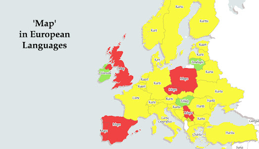

Disaster Ninja is a map of global population density correlated to OpenStreetMap density. It shows the number of OpenStreetMap objects mapped compared to the local population density. The map can therefore be used to quickly identify populated locations around the world which have not been fully mapped on OSM.

Disaster Ninja was initially developed to help disaster relief. The map can be used to quickly determine the level of OSM coverage compared to the local population after a natural disaster. It is therefore a useful tool for organizations such as the Humanitarian OpenStreetMap Team, who develop and use OSM map data as part of their disaster response and management efforts.

The Disaster Ninja interactive map uses a bivariate choropleth overlay to show the number of OSM map objects compared to the population per kilometer squared. The red areas on the map are locations which have a high population density and a low number of mapped objects on OSM. The red areas on the map are therefore locations which are likely to not be fully mapped on OpenStreetMap. At the other end of the bivariate scale are the light green areas. These are locations with a relatively small population and a large number of mapped objects.

At a glance India and China seem to be two areas of the world with a relatively high population density and low OSM map object count. The very high population densities in some areas of these countries may partly account for this. However some of the most densely populated areas, such as New Delhi, Mumbai and Beijing actually show up as green on the map and are therefore relatively well mapped on OSM.

Via: Weekly OSM

Map in European Languages


The map above shows the word 'map' translated into a number of different European languages. The continent is mostly divided between those who derive the word 'map' from Latin and those who derive the word from Greek.

The word for 'map' in English, Spanish, Portuguese, Polish, Czech and Serbian comes from the Latin 'mappa' for 'sheet' or 'napkin'. The word's use to describe a drawn representation of an area originates from the medieval Latin 'mappa mundi'. The literal translation of 'mappa mundi' is 'sheet of the world', from Latin mappa ‘sheet, napkin’ and mundi ‘of the world’ (genitive of mundus ).

Most other languages in Europe derive the word 'map' from the Greek word 'khártēs' (meaning map). These include the French, who use 'Carte', the German 'Karte' and the Danish 'Kort'.

In English, despite using a Latin derived word as the name for a map, we use a Greek word for the science or practice of drawing maps. The word 'cartography' comes from the French 'cartographie', from Ancient Greek 'khártēs' (map) + 'gráphō' (write). The other users of the Latin 'mappa' to describe a map (Spain, Portugal, Poland, Czechia and Serbia) also use a word derived from these Greek words (khártēs+'gráphō) to describe the actual science of making maps.

Sunday, July 14, 2019

City Neighborhood Quiz

How well do you know your global cities? Could you name a city just from a list of its central neighborhoods? Let's find out.

The maps below have had all road and building data removed. In fact the only thing left on these maps are the place-name labels of each city's central neighborhoods / boroughs. All you have to do is identify the city featured in each of the maps.

There are seven cities to guess in total.

1.

2.

3.

4.

5.

6.

7.


Answers (highlight the text below to reveal the answers)

1. London
2. New York
3. Paris
4. Berlin
5. San Francisco
6. Los Angeles
7. Sydney